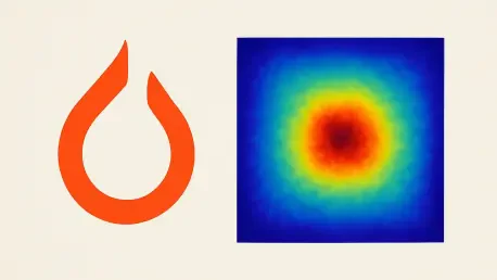

The structural opacity inherent in deep neural networks remains a significant barrier to their widespread adoption in high-stakes environments where transparency and accountability are non-negotiable. Setting a neural network to evaluation mode is a prerequisite for saliency computation because it disables stochastic operations like dropout that would otherwise interfere with gradient stability. As the industry moves further into 2026, the demand for explainable artificial intelligence (XAI) has transitioned from a theoretical preference to a strict regulatory and functional requirement across many sectors. Saliency maps have emerged as a cornerstone technique in this domain, providing a visual mechanism to audit the decision-making process of complex architectures. By calculating the gradients of a specific output class with respect to the input pixels, these maps offer a window into what a model “sees” when it classifies an image. This capability is essential for detecting spurious correlations, where a model might achieve high accuracy by focusing on background noise or watermarks rather than the actual subject of interest. Utilizing robust frameworks like PyTorch and specialized libraries such as Captum allows developers to implement these diagnostic tools with a high degree of precision and mathematical rigor, ensuring that the insights derived are both actionable and scientifically sound for production environments.
1. Load Modules and Initialize the Model
The initial phase of any interpretability workflow involves assembling the necessary computational tools and preparing the model for a forensic examination of its internal logic. In the current landscape of 2026, PyTorch serves as the primary backbone for these operations, offering the flexibility required to intercept and analyze gradient flow across various layers. To begin, one must import the core torch library alongside Torchvision, which provides access to industry-standard pre-trained models like ResNet-50. These architectures serve as excellent benchmarks for saliency research due to their well-documented performance and hierarchical feature extraction capabilities. Furthermore, the integration of Captum is indispensable, as it provides a suite of advanced attribution algorithms designed to simplify the complexities of model interrogation. The preparation process starts with loading a model that has already been trained on a massive dataset, such as ImageNet, which ensures that the features being analyzed are representative of real-world visual patterns and complex semantic relationships rather than random noise or initialization artifacts.
Transitioning the model into the correct operational state is a critical step that often determines the validity of the resulting attribution data. Using the model.eval() method ensures that every layer within the architecture behaves deterministically, which is vital for a process that relies on precise gradient calculations. In a training context, layers such as dropout randomly deactivate neurons to prevent overfitting, and batch normalization layers track running statistics that fluctuate with every batch. While these behaviors are beneficial for learning, they introduce unwanted noise and inconsistency when one is attempting to isolate the influence of specific input features on a single prediction. By locking the model into its evaluation mode, the system provides a stable environment where the gradients represent a fixed snapshot of the model’s knowledge. The following code demonstrates the standard procedure for initializing a ResNet-50 architecture and ensuring it is ready for the saliency computation pipeline, establishing a reliable foundation for the subsequent analytical steps of the project:
import torchimport torchvision.models as modelsfrom captum.attr import Saliencyfrom captum.attr import visualization as vizimport numpy as npmodel = models.resnet50(pretrained=True)model.eval()2. Prepare the Input Tensor and Enable Gradient Tracking
Effective model interpretability requires data formatted to match the specific expectations of the neural network’s architecture. In modern computer vision tasks, this typically involves structuring the input as a four-dimensional tensor, which represents the batch size, the number of color channels, the height of the image, and its width. Standardizing these dimensions is not merely a formatting requirement but a prerequisite for the mathematical operations that occur during the forward and backward passes. For instance, a batch size of one is commonly used during single-image attribution to focus the analysis on a specific instance of prediction. The normalization of pixel values is equally important, as models like ResNet are sensitive to the mean and standard deviation of the data they were originally trained on. By meticulously preparing the input tensor, researchers ensure that the model processes the image naturally, without introducing artifacts that could skew the resulting saliency map or lead to misleading interpretations of feature importance in the final output.
Beyond the spatial dimensions of the data, the computational mechanics of saliency maps depend on the ability to track how changes in input pixels affect the final output score. This is achieved by explicitly enabling gradient tracking on the input tensor using the requires_grad=True flag. By default, input tensors are treated as fixed constants that do not require optimization, but saliency analysis treats the input as a variable. This allows the PyTorch autograd engine to build a computational graph that links the input directly to the output logits. When the system performs a backward pass, it calculates the partial derivative of the target class with respect to each individual pixel. This value represents the sensitivity of the model; if a small change in a pixel causes a large change in the prediction, that pixel is considered highly salient. The following example illustrates the creation of a synthetic input tensor that mimics the structure of a standard RGB image while preparing it for gradient-based attribution analysis within the interpretability framework:
input_tensor = torch.randn(1, 3, 224, 224, requires_grad=True)3. Set Up the Saliency Attribution Engine
The complexity of modern deep learning architectures necessitates using specialized attribution engines that can navigate the intricate layers of a model to extract meaningful insights. Captum’s Saliency class is specifically designed to handle this task by providing a streamlined interface for first-order gradient attribution. Unlike manual gradient calculation, which requires custom scripts to handle different model types and output layers, this attribution engine abstracts the underlying complexity, allowing for a consistent approach across diverse projects. This abstraction is particularly valuable when working with multi-branch architectures or models with unconventional activation functions. By creating a dedicated saliency object, the user establishes a direct link between the model’s forward function and the interpretability algorithms. This ensures that every calculation is performed using the most efficient paths available in the PyTorch backend, minimizing the overhead associated with large-scale data analysis and enabling real-time diagnostic workflows for developers.
Initializing the attribution engine is a straightforward yet pivotal moment in the interpretability pipeline, as it binds the analytical tool to the specific logic of the model. The engine acts as a wrapper that observes the model’s behavior without modifying its weights or architecture. This non-invasive approach is essential for maintaining the integrity of the research, as it ensures that the saliency map reflects the model’s actual state rather than a modified version created for visualization purposes. Furthermore, the modular nature of the engine allows it to be swapped out for more advanced methods, such as Integrated Gradients or DeepLIFT, as the needs of the project evolve during the research phase. By starting with the vanilla saliency engine, one establishes a baseline for understanding which regions of an image the model prioritizes during its inference cycle. The following code snippet demonstrates the simple instantiation of the saliency engine by passing the model as the primary argument, thereby creating a powerful tool for visual evidence gathering and model verification:
saliency_engine = Saliency(model)4. Generate the Attribution Values
Generating the actual attribution map requires identifying a specific target class, which directs the analytical focus toward a particular outcome the model is capable of predicting. In a classification model trained on a wide variety of categories, the target index corresponds to a specific label, such as a “Persian cat” or a “golden retriever.” This targeting is crucial because a single image may contain multiple objects, and the model’s reasons for identifying one object may differ significantly from its reasons for identifying another. By specifying a target class index, the attribution engine isolates the specific gradients associated with that class, ignoring the signals related to other potential labels. This precision allows researchers to verify if the model is correctly identifying the defining characteristics of a specific category or if it is being influenced by irrelevant features that happen to be present in the scene, thereby improving the diagnostic value of the generated heatmap for end-users.
The computation of these gradients often involves the use of the absolute value setting, which aggregates the positive and negative influences into a single magnitude of sensitivity. In the context of visual saliency, a pixel is important if it has a strong impact on the prediction, regardless of whether increasing its intensity makes the prediction more or less likely. By setting the abs=True parameter, the system produces a map where bright spots represent the areas of highest overall influence, creating a more intuitive visual guide for human observers. This step effectively collapses the directional data into a unified importance score, making it easier to see at a glance which part of the input image was most critical to the final decision. The following code demonstrates how to execute the attribution process for a specific target label, resulting in a raw data tensor that contains the fine-grained importance values for every pixel in the input image, ready for the final processing and visualization steps:
target_label = 281attribution_data = saliency_engine.attribute(input_tensor, target=target_label, abs=True)5. Reformat and Render the Heatmap
Raw attribution data generated by the engine is stored in a format optimized for GPU computation and tensor operations, which is often incompatible with standard image processing and visualization libraries. To bridge this gap, the data must be moved from the computational device—such as a CUDA-enabled GPU—back to the system’s central memory. Once the data is on the CPU, it is converted into a NumPy array, which is the universal format for numerical computing in Python. This conversion is accompanied by the detach() method, which removes the tensor from the computational graph, and the squeeze() method, which removes the batch dimension if it is no longer needed for the current analysis. Reordering the axes from a “channels-first” layout to a “channels-last” layout is another essential transformation. Standard imaging tools expect the color channels to be the final dimension of the array, and failing to perform this transposition would result in distorted or unreadable visual outputs that fail to represent the spatial relevance of the processed data.
The final visualization process uses specialized utilities to transform the numerical gradients into a human-readable heatmap that clearly highlights the most influential regions of the image. Captum provides a robust visualization library that handles normalization and color mapping automatically, ensuring that the resulting image is both visually appealing and scientifically accurate for reporting purposes. The heat_map method typically uses a color gradient where specific hues represent the intensity of the attribution, allowing for quick identification of the model’s focus areas. By adding a color bar, the visualization provides a quantitative reference for the relative importance of different pixels, which is vital for comparing results across different models or input images. This structured approach to rendering ensures that the technical findings are communicated effectively to stakeholders, regardless of their technical background. The following code illustrates the final steps of processing the attribution data and generating a clear visual representation of the model’s internal focus points:
processed_attr = np.transpose(attribution_data.squeeze(0).cpu().detach().numpy(), (1, 2, 0))fig, ax = viz.visualize_image_attr(attr=processed_attr,method='heat_map',sign='absolute_value',show_colorbar=True,title='Input Saliency Map')6. Advancing Machine Learning Transparency
The integration of saliency maps into the machine learning development lifecycle provided a critical layer of defense against the deployment of unreliable or biased models. By visualizing the specific input features that drove predictions, engineers identified significant flaws in data collection and model training that would have otherwise remained hidden within the layers of a black-box system. This proactive approach allowed for the refinement of datasets and the adjustment of architectural parameters before the models reached the production stage. As researchers looked toward the future of the field, the transition to more sophisticated attribution methods, such as Integrated Gradients and Guided Backpropagation, represented the logical next step for teams seeking to move beyond simple first-order sensitivity analysis. These advanced techniques offered a more nuanced view of feature importance by addressing the limitations of gradient saturation and high-frequency noise inherent in vanilla saliency methods.
Ultimately, the adoption of standardized interpretability tools like Captum fostered a culture of transparency and rigorous validation within the AI community. This move toward greater openness and auditability ensured that neural networks became not only more accurate but also more trustworthy as they integrated into the essential infrastructure of modern society. From 2026 to 2028, the industry established new protocols for model certification that mandated the inclusion of attribution maps in all technical documentation. These changes improved the collaborative potential between data scientists and domain experts, as visual heatmaps provided a common language for discussing model behavior. By grounding technical analysis in visual evidence, the community moved closer to achieving the goal of truly explainable artificial intelligence, where every prediction can be scrutinized and justified with mathematical and visual clarity. Moving forward, the focus should remain on developing tools that bridge the gap between complex algorithmic outputs and human-centric understanding.